Continuous Thought Machines
Neural Synchronization for Emergent Intelligence
Luke Darlow, Ciaran Regan, Sebastian Risi, Jeffrey Seely, Llion Jones
Sakana AI
May 2025
Executive Summary
This paper introduces Continuous Thought Machines (CTM), a revolutionary neural architecture that treats temporal dynamics as a fundamental computational primitive rather than an abstraction to be eliminated. Unlike standard neural networks that process information in discrete, static layers, CTMs allow "thought" to unfold over an internal time dimension, using neural synchronization patterns as the core representation for taking actions.
The results are remarkable: CTMs achieve 6× generalization beyond training distribution on maze navigation (trained on 39×39, solves 99×99), demonstrate near-perfect accuracy on cumulative parity where LSTMs fail, show better-than-human calibration on image classification, and exhibit emergent behaviors like adaptive compute allocation and interpretable "thinking" trajectories—all without explicitly designing for these capabilities.
The key insight is that by allowing neurons to maintain individual temporal histories and learn per-neuron dynamics through Neuron-Level Models (NLMs), CTMs bridge computational efficiency with biological plausibility, opening new research directions for systems exhibiting more human-like intelligence.
🎯 ELI5: What is a Continuous Thought Machine?
Imagine your brain as an orchestra. In a standard neural network, every musician plays their note simultaneously in one instant—there's no melody, just a single chord. In a Continuous Thought Machine, the orchestra plays over time: violins start, then cellos join in, patterns emerge between instruments, and the final piece emerges from how they synchronize together over time. The CTM watches which neurons "fire together" across time and uses that synchronization pattern—not just the final notes—to make decisions. This is closer to how real brains work, where timing and rhythm of neural activity carry meaningful information.
Part 1: The Core Innovation—Time as Computation
Standard neural networks treat computation as instantaneous: input goes in, activations propagate through layers, output comes out. Time exists only for processing sequential data. But this fundamentally differs from biological neural systems, where when a neuron fires matters as much as whether it fires.
The Three Pillars of CTM Architecture
1. Decoupled Internal Time Dimension
CTM introduces an internal recurrence timeline t ∈ {1,...,T} that is completely independent from any sequential data structure. Even for a single static image, the CTM processes it over multiple internal "ticks," allowing iterative refinement of representations. This internal time enables the model to "think" about inputs rather than just react to them.
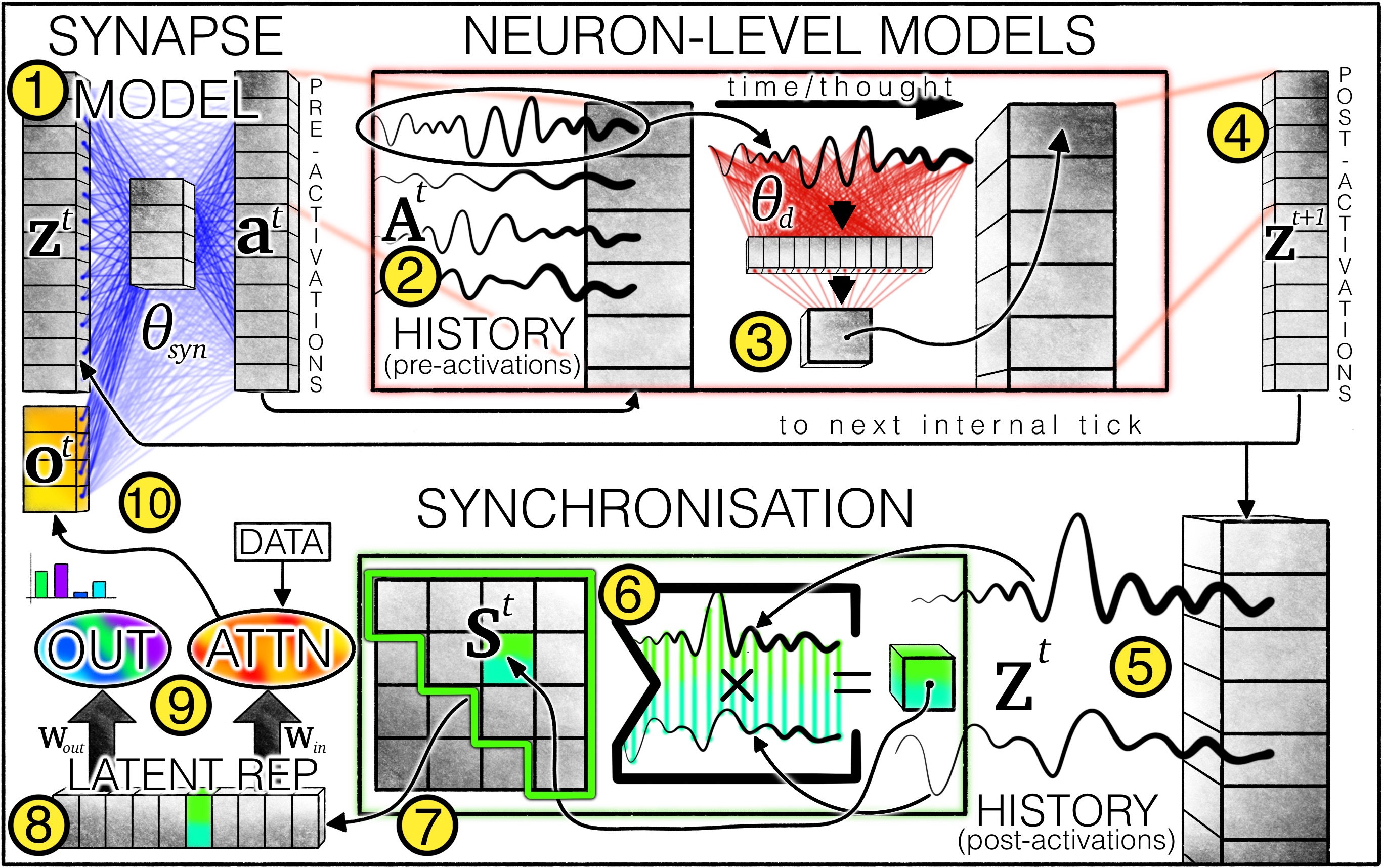
2. Neuron-Level Models (NLMs)
Each neuron receives its own private MLP that processes its historical pre-activations. Unlike standard recurrent networks where all neurons share the same recurrence weights, NLMs allow each neuron to develop its own unique temporal dynamics. This is analogous to how biological neurons have different time constants and response properties.
3. Synchronization-Based Representation
Rather than using raw activations, CTM computes a synchronization matrix St = Zt · (Zt)⊺ that captures how pairs of neurons correlate over time. This matrix—representing which neurons "fire together"—is the fundamental representation used for outputs and attention. This mirrors biological findings that neural synchronization carries meaningful information.
Mathematical Formulation
Pre-activations: at = fθsyn(concat(zt, ot)) ∈ ℝD
Post-activations: zd(t+1) = gθd(Adt) — each neuron has its own NLM gθd
Synchronization: St = Zt · (Zt)⊺ ∈ ℝD×D
History maintained as FIFO lists of length M for each neuron
🧬 Biological Inspiration
The CTM architecture draws from multiple neuroscience principles:
- Spike-Timing-Dependent Plasticity (STDP): Learning depends on precise timing relationships between neural firing
- Neural Oscillations: Brain rhythms (gamma, theta, alpha) coordinate information processing
- Temporal Coding: Information encoded in when neurons fire, not just firing rates
- Traveling Waves: Activity patterns propagate spatially through neural tissue
Part 2: The Training Dynamics—Learning When to Decide
A critical innovation in CTM is how it handles training across internal time steps. Rather than forcing the network to produce correct outputs at a fixed time, CTM dynamically selects the optimal moments for evaluation.
Dynamic Loss Selection
The CTM training objective combines two key time points:
t1 = argmint(Lt) — the tick with minimum loss
t2 = argmaxt(Ct) — the tick with maximum certainty
Final Loss: L = (Lt₁ + Lt₂) / 2
Why This Matters: Curriculum Learning Emerges Naturally
This loss formulation creates emergent curriculum learning. Early in training, easy examples achieve low loss quickly (low t1), while hard examples need more internal steps. As training progresses, the model learns to use more internal computation for difficult inputs and less for easy ones. The certainty term (t2) ensures the model develops confidence in its decisions.
Part 3: ImageNet Classification—Seeing Models Think
The first major experiment applies CTM to ImageNet classification, revealing interpretable "thinking" processes and exceptional calibration properties.
Interpretable Attention Patterns
Unlike black-box models, CTM's attention maps reveal how the model processes images over time. The attention starts broad, covering the entire image, then progressively focuses on discriminative regions. This mirrors human visual attention: we first take in the whole scene, then focus on relevant details.
Better-Than-Human Calibration
On CIFAR-10, CTM achieves calibration superior to human performance. When the model says it's 80% confident, it's correct 80% of the time. This is crucial for real-world deployment where knowing when you don't know is as important as knowing the answer.
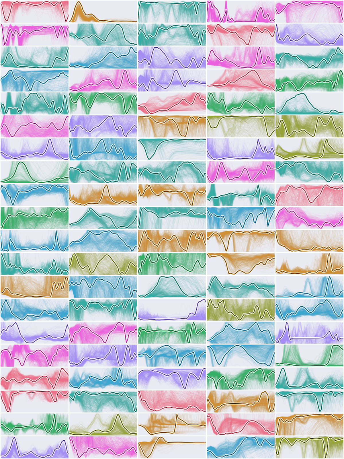
Neural Dynamics Visualization
When visualizing CTM neuron activations over time, rich dynamics emerge spontaneously:
CTM Dynamics
Shows periodic activity, traveling waves, and multi-scale temporal structure—all without any explicit design for periodicity. Different neurons develop different characteristic patterns.
LSTM Dynamics
Shows relatively monotonic evolution toward a fixed point. Less temporal structure and diversity across neurons.
Part 4: Maze Navigation—Building World Models
The maze navigation task demonstrates CTM's ability to build internal world models and generalize far beyond training distribution.
Extraordinary Generalization
6× Beyond Training Distribution
CTMs trained on 39×39 mazes (path lengths ~100) successfully solve 99×99 mazes—a 6× increase in problem complexity. This isn't just slight extrapolation; it's solving fundamentally larger problems than ever seen in training.
How Does It Work? Internal World Model
Analysis of the attention patterns reveals that CTM builds an internal world model of the maze. The attention literally traces the solution path from start to finish, showing the model has learned the underlying structure of maze navigation rather than memorizing patterns.
No Positional Encoding Required
Unlike Transformers that require explicit positional encodings, CTM solves mazes without any position information. The temporal dynamics themselves provide the necessary structure for understanding spatial relationships. This suggests the internal time dimension serves as a universal computational scaffold.
Part 5: Cumulative Parity—Testing Algorithmic Reasoning
The cumulative parity task tests whether models can perform sequential algorithmic reasoning: given a sequence of bits, output the running XOR at each position.
| Model |
Internal Ticks |
Final Accuracy |
Notes |
| LSTM |
N/A |
~20% |
Struggles regardless of capacity |
| CTM |
10 |
~40% |
Insufficient thinking time |
| CTM |
25 |
~70% |
Improving with more ticks |
| CTM |
75+ |
~100% |
Near-perfect performance |
Emergent Planning Behavior
Backward Attention—The Model Plans Ahead
Analysis of attention patterns reveals something striking: the CTM's attention moves backward through the sequence. Instead of processing left-to-right like typical sequential models, CTM appears to "plan" by looking ahead to upcoming bits. This emergent bidirectional processing wasn't designed—it emerged from the architecture's freedom to allocate attention over internal time.
Part 6: Q&A MNIST—Memory and Reasoning
The Q&A MNIST task tests memory: the model sees a sequence of digit images, then must answer questions like "What was the 3rd digit?" or "Was any digit greater than 5?"
Generalization to Longer Sequences
The generalization grids reveal how well models trained on shorter sequences perform on longer ones:
CTM (10 internal ticks)
Strong generalization pattern with high accuracy maintained across sequence length variations. The synchronization-based memory provides robust recall.
LSTM (10 internal ticks)
Performance degrades more rapidly with increased sequence length. Traditional recurrent memory struggles with out-of-distribution lengths.
Part 7: Sorting Numbers—Adaptive Computation
The sorting task reveals CTM's ability to allocate computation adaptively based on problem difficulty.
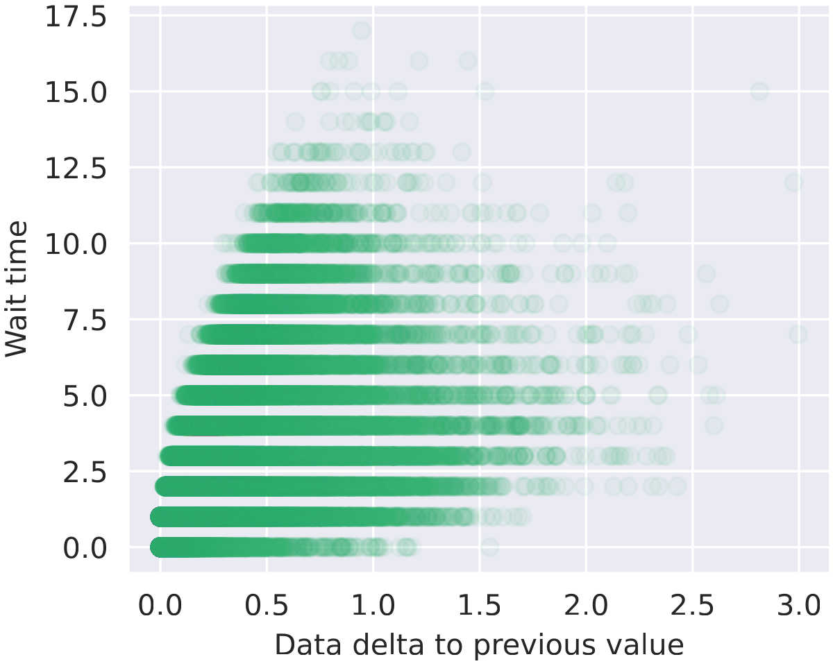
Emergent Difficulty Estimation
The Model Knows What's Hard
Analysis reveals that CTM's "wait time" before outputting each sorted element correlates with the gap between consecutive sorted values. When two numbers are close together (harder to order), the model takes more internal ticks to decide. When numbers are far apart (easy), it decides quickly. This difficulty-aware computation wasn't trained—it emerged naturally.
Part 8: Ablation Studies—What Really Matters?
Model Width and Neuron Diversity
Analysis of neuron similarity reveals why width helps: wider models develop more diverse neuron behaviors. With more neurons, each can specialize for different temporal patterns, creating a richer representational space.
Internal Ticks and Accuracy
Key Findings from Ablations
- More ticks = better accuracy up to a task-dependent ceiling (15-25 for images, 75+ for algorithmic tasks)
- Wider models develop more diverse neurons with different temporal response patterns
- NLM history length M provides diminishing returns beyond M=8-16
- Synchronization matrix is essential—removing it dramatically hurts performance
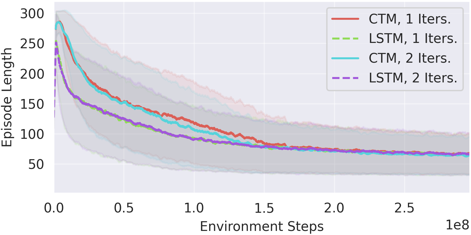
Part 9: Reinforcement Learning—Continuous-Time Agents
CTM extends to reinforcement learning, maintaining continuous activation histories across environment steps.
The key insight is that CTM's internal time can persist across environment steps, allowing the agent to maintain "trains of thought" that span multiple actions. This is more biologically plausible than resetting hidden states at each step.
Part 10: Implications and Future Directions
What CTM Teaches Us About Intelligence
Time Is Not Just a Convenience—It's Computational
The success of CTM suggests that temporal dynamics are not merely a biological quirk to be abstracted away, but a fundamental computational resource. By allowing information to evolve over internal time, CTM achieves capabilities that elude architectures treating computation as instantaneous:
- Adaptive computation: Harder problems automatically get more processing
- Emergent planning: Backward attention enables looking ahead
- World models: Internal simulations build without explicit design
- Calibration: Uncertainty estimation arises from temporal uncertainty
Comparison to Other Approaches
| Feature |
Standard NN |
LSTM/RNN |
Transformer |
CTM |
| Internal computation time |
Fixed (depth) |
Tied to sequence |
Fixed (layers) |
Adaptive |
| Per-neuron dynamics |
No |
No (shared weights) |
No |
Yes (NLMs) |
| Synchronization representation |
No |
No |
Partial (attention) |
Yes |
| Biological plausibility |
Low |
Medium |
Low |
High |
| Interpretability |
Low |
Medium |
Medium |
High |
Future Research Directions
Open Questions and Opportunities
Scaling: How do CTM properties change with model size? Do emergent behaviors become more sophisticated?
Language: Can CTM's temporal dynamics improve language model reasoning and calibration?
Multimodal: Does synchronization provide natural binding for multimodal representations?
Continual Learning: Can persistent temporal dynamics enable better lifelong learning?
Neuroscience: Do CTM dynamics predict biological neural phenomena?
Conclusion
Continuous Thought Machines represent a fundamental rethinking of neural network computation. By embracing temporal dynamics rather than abstracting them away, CTM achieves:
- 6× generalization beyond training distribution on maze navigation
- Near-perfect accuracy on algorithmic tasks where LSTMs fail
- Better-than-human calibration on image classification
- Emergent adaptive computation matching difficulty to thinking time
- Interpretable processing with visible attention trajectories
The key insight is that neural synchronization—how neurons fire together over time—provides a rich representational space that standard architectures miss. Rather than computing instant answers, CTMs think about their inputs, developing answers through temporal evolution.
For practitioners: CTM suggests that adding internal recurrence with per-neuron dynamics can unlock capabilities beyond what static architectures achieve. The success of synchronization-based representations hints at fundamentally new approaches to representation learning.
For researchers: This work opens a new paradigm where time is a first-class computational citizen. The emergent behaviors—planning, calibration, adaptive compute—suggest we're just scratching the surface of what temporal neural architectures can achieve.