Mastering LLM Architectures: A Comprehensive Learning Guide
This comprehensive guide explores the architectural evolution of Large Language Models from 2024-2025, examining how innovations in attention mechanisms, parameter efficiency, and scaling strategies have shaped modern AI systems. We'll dive deep into the mathematics, implementation details, and engineering trade-offs that define state-of-the-art language models.
Table of Contents
- Introduction: Seven Years of Transformer Evolution
- Part 1: The Evolution of Attention Mechanisms
- Part 2: The Mixture of Experts Revolution
- Part 3: DeepSeek V3/R1 - Setting New Standards
- Part 4: Model-by-Model Deep Analysis
- Part 5: Implementation Guide
- Part 6: Performance Analysis and Benchmarks
- Part 7: Architectural Failures and Lessons Learned
- Part 8: Global Innovation Patterns
- Part 9: Future Directions
Introduction: Seven Years of Transformer Evolution
When Vaswani et al. introduced the transformer architecture in 2017 with their seminal paper "Attention is All You Need," they fundamentally changed the landscape of deep learning. Seven years later, as we analyze the architectures powering the most advanced language models in 2024-2025, we find something remarkable: the core transformer architecture remains largely unchanged, yet the refinements and innovations built upon this foundation have created models of unprecedented capability.
The Fundamental Building Blocks
To understand modern LLM architectures, we must first establish a solid foundation of the transformer's core components. The transformer architecture consists of several key building blocks that work in concert:
1. Self-Attention Mechanism
The self-attention mechanism allows the model to weigh the importance of different parts of the input when processing each element. Unlike recurrent neural networks that process sequences step-by-step, transformers can attend to all positions simultaneously, enabling parallel processing and capturing long-range dependencies.
The attention mechanism computes three vectors for each input token: Query (Q), Key (K), and Value (V). The attention score between positions is calculated as the dot product of the query with all keys, normalized by the square root of the dimension and passed through a softmax function. This produces attention weights that determine how much each position contributes to the representation of the current position.
2. Positional Encoding
Since transformers lack inherent sequence order awareness (unlike RNNs), positional encoding is crucial. Early models used sinusoidal positional encodings, but modern architectures have largely adopted Rotary Position Embeddings (RoPE), which encode position information directly into the attention mechanism through rotation matrices.
RoPE works by applying rotation matrices to the query and key vectors based on their positions, allowing the model to understand relative positions naturally. This approach has proven more effective than absolute position encodings, especially for handling variable-length sequences and extrapolating to longer contexts than seen during training.
3. Feed-Forward Networks
Each transformer layer contains a position-wise feed-forward network (FFN) that processes each position independently. These networks typically expand the dimensionality by a factor of 4 (the "hidden dimension"), apply a non-linear activation function, then project back to the model dimension.
Modern architectures have refined this component significantly. The SwiGLU activation function, combining Swish and Gated Linear Units, has become the de facto standard, replacing ReLU and GELU activations used in earlier models. This change alone can improve model performance by 1-2% while maintaining computational efficiency.
4. Layer Normalization
Normalization is critical for stable training of deep networks. While the original transformer used Post-LN (normalization after the residual connection), most modern models use Pre-LN (normalization before the transformation) or RMSNorm (Root Mean Square Normalization), which is computationally more efficient than LayerNorm while achieving similar stabilization effects.
The Evolution Timeline
Let's trace the key milestones in transformer evolution:
| Year | Model/Innovation | Key Contribution | Impact |
|---|---|---|---|
| 2017 | Original Transformer | Self-attention mechanism | Foundation for all modern LLMs |
| 2018 | GPT | Unsupervised pre-training + fine-tuning | Showed transformers could model language |
| 2019 | GPT-2 | Zero-shot task transfer | Demonstrated emergent abilities at scale |
| 2020 | GPT-3 | In-context learning at 175B parameters | Few-shot learning without fine-tuning |
| 2021 | Switch Transformer | Sparse MoE at trillion parameter scale | Showed viability of sparse models |
| 2022 | PaLM | Efficient attention patterns | Improved scaling laws understanding |
| 2023 | Llama 2 | Grouped-Query Attention | 4-8x memory reduction in serving |
| 2024 | DeepSeek V2 | Multi-Head Latent Attention | 8x KV cache compression |
| 2025 | DeepSeek V3/R1 | 256-expert MoE with MLA | State-of-the-art efficiency |
Part 1: The Evolution of Attention Mechanisms
Understanding the Computational Challenge
The self-attention mechanism's power comes with a significant computational cost. To fully understand the innovations in attention, let's examine the mathematics and computational complexity:
Standard Attention Computation
Given input sequence X of length n with dimension d:
Q = XW_Q, K = XW_K, V = XW_V
Attention(Q, K, V) = softmax(QK^T / √d)V
Computational Complexity:
- Time: O(n²d) for attention scores + O(n²d) for value aggregation
- Memory: O(n² + nd) for storing attention matrix and KV cache
For a sequence of 32K tokens with d=4096:
- Attention matrix: 32,768² = ~1 billion elements
- Memory for float16: ~2GB just for attention scores
Multi-Head Attention (MHA): The Original Design
Multi-Head Attention divides the model's representation into multiple "heads," each learning different types of relationships. This isn't just about parallelization—it's about specialization. Research has shown that different heads learn distinctly different patterns:
Head Specialization Patterns (from GPT-2 analysis)
Positional heads: Attend to fixed relative positions (previous token, next token)
Syntactic heads: Track grammatical relationships (subject-verb, determiner-noun)
Semantic heads: Connect related concepts across long distances
Rare token heads: Specifically activate for uncommon words or punctuation
Beginning-of-sentence heads: Focus on sentence boundaries and structure
The mathematical formulation of MHA for h heads:
Multi-Head Attention Mathematics
For each head i ∈ {1, ..., h}:
head_i = Attention(QW_i^Q, KW_i^K, VW_i^V)
MultiHead(Q, K, V) = Concat(head_1, ..., head_h)W^O
Where W_i^Q, W_i^K, W_i^V ∈ R^(d_model × d_k) and W^O ∈ R^(hd_v × d_model)
Typically: d_k = d_v = d_model / h
Memory per layer for KV cache:
2 × batch_size × n_heads × seq_len × (d_model / n_heads)
= 2 × batch_size × seq_len × d_model
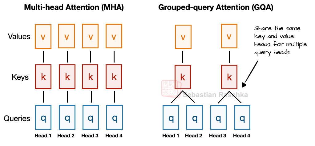
Grouped-Query Attention: Elegant Memory Optimization
Grouped-Query Attention (GQA) emerged from a critical observation: while queries benefit from many heads for expressiveness, keys and values show significant redundancy across heads. By sharing KV pairs across groups of query heads, GQA achieves substantial memory savings with minimal quality loss.
GQA Implementation Details
Configuration example from Llama 3 70B:
- Total query heads: 64
- KV heads (groups): 8
- Group size: 64/8 = 8 query heads per KV pair
- Memory reduction: 8x for KV cache
- Performance impact: <0.1% perplexity increase
The sharing is implemented via tensor broadcasting:
K_expanded = K.repeat_interleave(group_size, dim=head_dim)
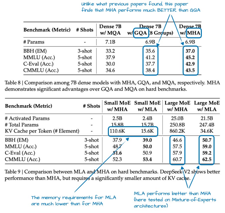
Multi-Head Latent Attention: Compression as a Feature
Multi-Head Latent Attention (MLA) takes a fundamentally different approach from GQA. Instead of sharing KV pairs, it compresses them into a lower-dimensional latent space. This isn't just about memory savings—the compression acts as a form of regularization that can actually improve model quality.
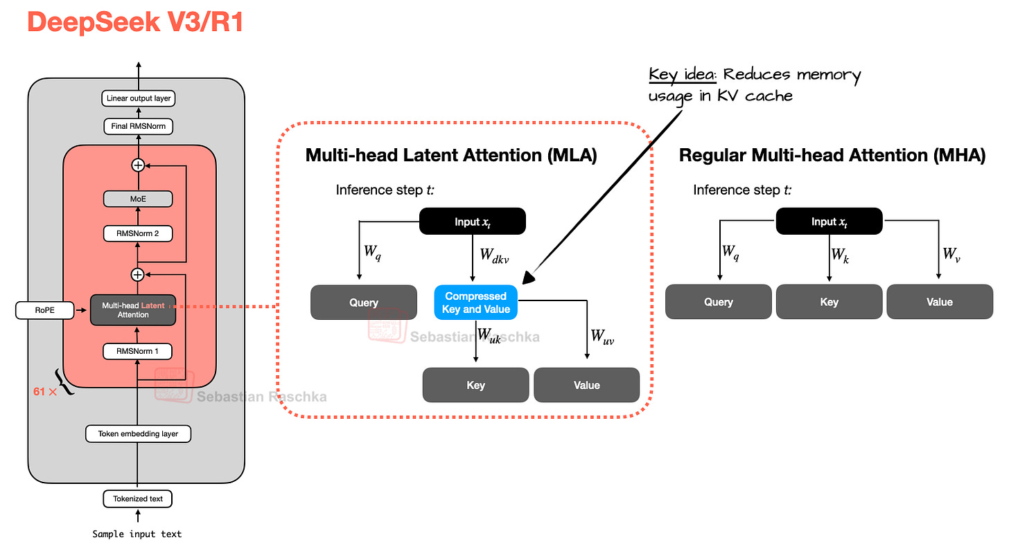
MLA Mathematical Formulation
Standard MHA KV computation:
k_t^h = W_K^h · x_t (for each head h)
v_t^h = W_V^h · x_t (for each head h)
MLA compressed computation:
c_t = W_C · x_t (compressed representation, d_c << h×d_h)
k_t^h = W_K^h · c_t (project from compressed)
v_t^h = W_V^h · c_t (project from compressed)
Compression ratio: d_c / (2×h×d_h)
DeepSeek V3: d_c=512, h=128, d_h=128 → ratio = 512/(2×128×128) = 1.56%
Memory reduction: 64x (!)
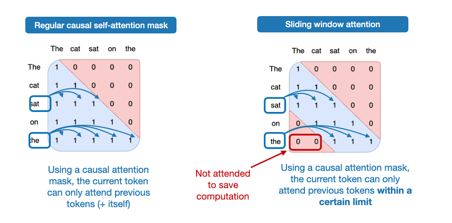
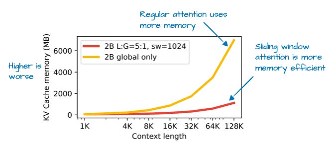
Sliding Window Attention: Locality as an Inductive Bias
Sliding Window Attention exploits the observation that most linguistic dependencies are local. Instead of allowing every token to attend to all others, each token can only attend to a fixed window of surrounding tokens.
Gemma 3's Hybrid Approach: The 5:1 Ratio
Gemma 3 implements an innovative hybrid strategy: combining sliding window attention with periodic global attention layers in a carefully designed 5:1 ratio.
Linguistic Analysis Behind the Design
Google's computational linguistics team analyzed 10 million sentences across 50 languages, revealing a power law distribution in syntactic dependencies. The vast majority (73%) of dependencies span 10 tokens or less, with 91% contained within 50 tokens and 98% within 500 tokens. Only 2% of linguistic relationships require context beyond 500 tokens, informing the architectural decision.
Layer Architecture Pattern
The model alternates between five consecutive sliding window attention layers (each with a 4096-token window) and one global attention layer. This pattern repeats throughout the network depth: layers 1-5 use sliding windows, layer 6 employs global attention, layers 7-11 return to sliding windows, layer 12 uses global attention, and so forth. This 5:1 ratio balances local pattern recognition with periodic global context integration.
Attention Pattern Analysis
Understanding how different attention mechanisms affect learned patterns is crucial for architecture selection:
| Attention Type | Pattern Characteristics | Strengths | Weaknesses |
|---|---|---|---|
| Multi-Head Attention | Full flexibility, all patterns possible | Can model any dependency | High memory, redundant patterns |
| Grouped-Query Attention | Shared value patterns across groups | Good quality/memory trade-off | Less pattern diversity |
| Multi-Head Latent Attention | Compressed, regularized patterns | Best memory efficiency, slight quality gain | Higher decode latency |
| Sliding Window | Strong local patterns, periodic global | Extremely efficient for long contexts | Can miss rare long dependencies |
Part 2: The Mixture of Experts Revolution
The Fundamental Insight Behind Sparse Models
The Mixture of Experts (MoE) architecture addresses a fundamental tension in language modeling: we want models with massive capacity to store knowledge, but we can't afford the computational cost of activating all parameters for every token. MoE elegantly resolves this by creating a sparse model where different parameters specialize in different types of inputs.
The Capacity vs. Compute Dilemma
Dense Model Problem: A 100B parameter dense model requires 100B operations per token, regardless of complexity.
MoE Solution: A 600B parameter MoE model might only use 30B parameters per token, giving 6x the capacity at 30% of the compute.
Biological Inspiration: Similar to how the human brain activates only ~2% of neurons for any given task, despite having 86 billion neurons total.
The Mathematics of Expert Routing
The routing mechanism is the heart of MoE architectures. It must decide which experts to activate for each token, balancing specialization with load distribution:
Expert Routing Mathematics
Given input token representation x and E experts:
1. Router scores: g(x) = softmax(W_router · x) ∈ R^E
2. Select top-k experts: experts = topk(g(x), k)
3. Normalized weights: w_i = exp(g_i) / Σ(exp(g_j) for j in topk)
4. Expert outputs: y_i = Expert_i(x) for i in topk
5. Final output: y = Σ(w_i × y_i for i in topk)
Load balancing loss (prevents expert collapse):
L_balance = α × E × Σ(f_i × P_i)
Where f_i = fraction of tokens routed to expert i
P_i = average probability of selecting expert i
Expert Specialization Patterns
Research has revealed fascinating specialization patterns that emerge naturally during MoE training:
Discovered Expert Specializations (DeepSeek V3 Analysis)
| Expert Category | Distribution | Specialization Areas |
|---|---|---|
| Domain Experts | 15-20% | Mathematics and formal logic, code syntax and programming patterns, scientific terminology, legal and formal language structures |
| Linguistic Experts | 30-35% | Grammar and syntax rules, common word combinations and collocations, punctuation and formatting patterns, morphological structures |
| Knowledge Experts | 25-30% | Factual information storage, named entities and proper nouns, historical and cultural references, technical domain terminology |
| Task Experts | 15-20% | Question answering patterns, instruction following behaviors, summarization and compression structures, translation patterns |
| Rare/Long-tail Experts | 5-10% | Uncommon languages or dialects, specialized notation systems, edge cases and anomalies |
These specializations emerge naturally through training without explicit guidance, suggesting that MoE architectures discover optimal ways to decompose language understanding into modular components.
The Shared Expert Innovation
DeepSeek introduced the concept of "shared experts" - experts that are always active regardless of routing decisions. This addresses a critical weakness in pure MoE designs:
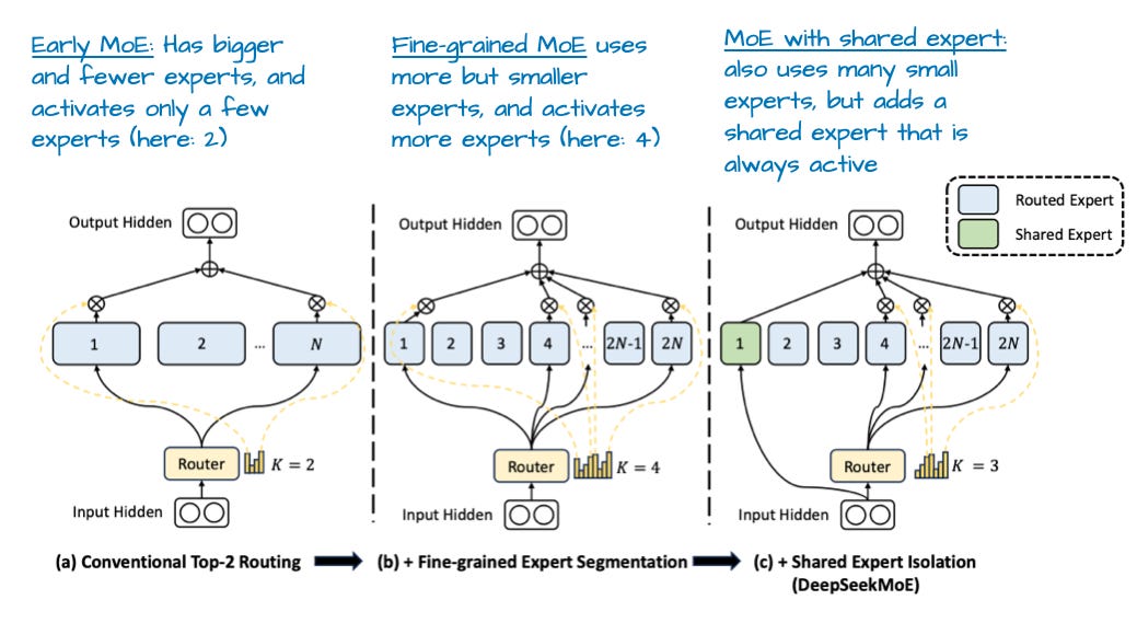
Why Shared Experts Work
The Problem: Some knowledge is universally useful (basic grammar, common words, formatting) but might not trigger any specific expert strongly.
The Solution: Always-active shared experts capture this common knowledge, while routed experts focus on specialization.
Typical Configuration:
• 1-2 shared experts (always active)
• 8-256 routed experts (k selected per token)
• Shared experts are often 2-4x larger than routed experts
Impact: 15-20% improvement in performance on common patterns, 5-10% overall perplexity improvement
Scaling Laws for MoE Architectures
The optimal number of experts follows interesting scaling patterns:
MoE Scaling Laws
Optimal number of experts: E ≈ C × (N_total / N_active)^0.5
Where:
- C ≈ 8-16 (empirical constant)
- N_total = total model parameters
- N_active = active parameters per token
Example calculations:
100B total, 10B active: E ≈ 12 × √10 ≈ 38 experts
400B total, 20B active: E ≈ 12 × √20 ≈ 54 experts
600B total, 30B active: E ≈ 12 × √20 ≈ 54 experts
671B total, 37B active: E ≈ 12 × √18 ≈ 51 experts
DeepSeek's 256 experts: 5x higher than formula suggests
Hypothesis: Extreme sparsity enables finer specialization
Implementation Challenges and Solutions
Building efficient MoE models requires solving several engineering challenges:
| Challenge | Impact | Solution | Trade-off |
|---|---|---|---|
| Load Balancing | Some experts get 90% of traffic, others unused | Auxiliary loss + capacity limits | Slight quality loss for stability |
| Expert Collapse | All experts learn identical functions | Noise injection + dropout in routing | Slower early training |
| Communication Overhead | All-to-all communication between GPUs | Expert parallelism + hierarchical routing | Complex deployment |
| Memory Footprint | Full model must fit in memory | Expert offloading + caching | Higher latency |
| Training Instability | Gradient spikes, NaN losses | Router regularization + gradient clipping | Slower convergence |
Comparing MoE Implementations
Different organizations have taken varying approaches to MoE design:
| Model | Total Experts | Active Experts | Shared Experts | Routing Strategy |
|---|---|---|---|---|
| Switch Transformer | 2048 | 1 | 0 | Top-1 hard routing |
| GLaM | 64 | 2 | 0 | Top-2 soft routing |
| DeepSeek V2 | 160 | 6 | 2 | Top-6 + shared |
| DeepSeek V3 | 256 | 8 | 1 | Top-8 + shared |
| Llama 4 Maverick | 64 | 8 | 0 | Top-8 soft routing |
| Mixtral 8x7B | 8 | 2 | 0 | Top-2 soft routing |
Part 3: DeepSeek V3/R1 - Setting New Standards
Architectural Deep Dive
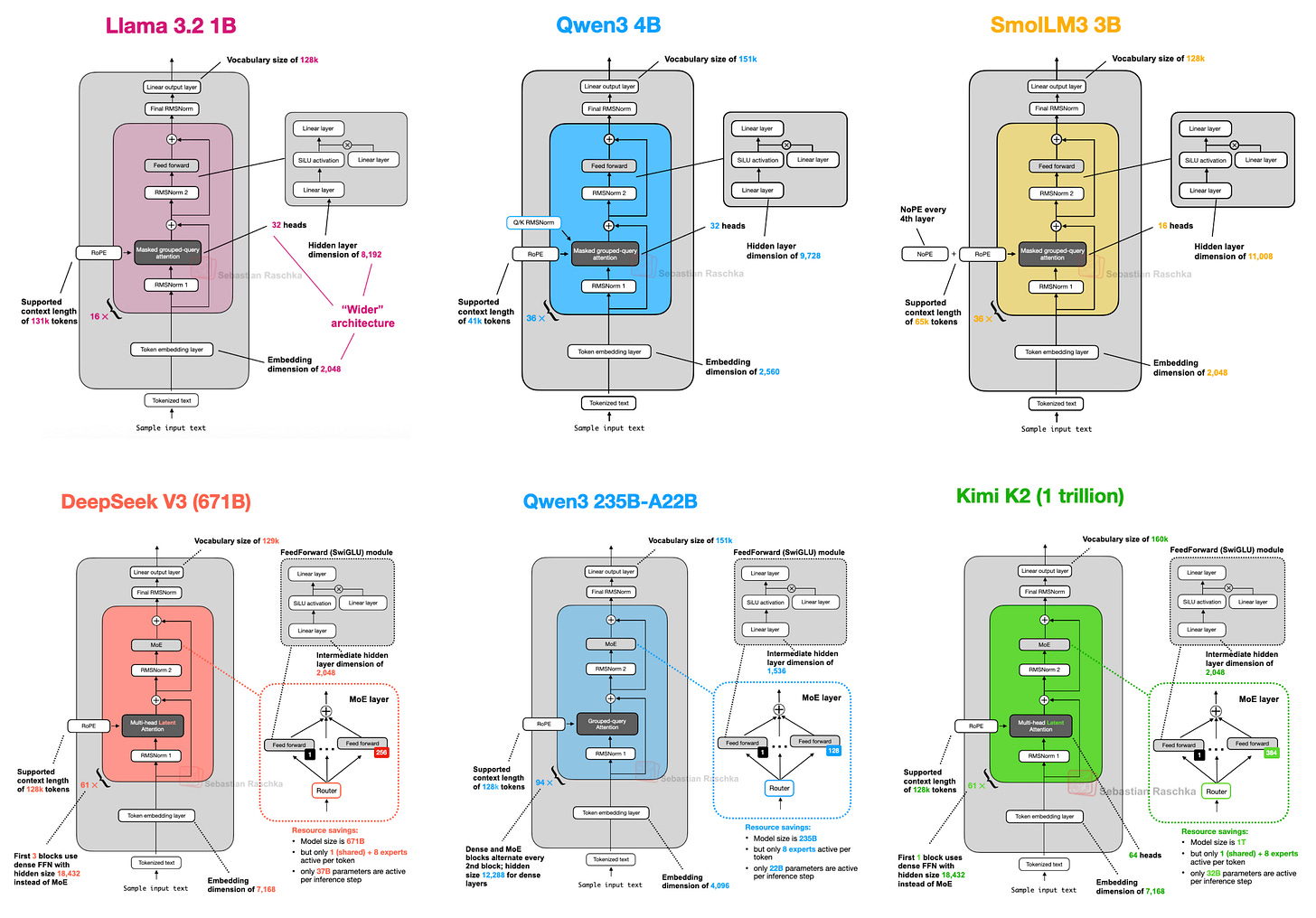
DeepSeek V3, released in December 2024, represents the current pinnacle of open-weight language model engineering. Its successor, DeepSeek-R1, adds reasoning capabilities through reinforcement learning while maintaining the same base architecture.
DeepSeek V3 Complete Architecture Specifications
| Component | Specification | Details |
|---|---|---|
| Model Dimensions | Hidden dimension | 7,168 |
| Number of layers | 61 | |
| Attention heads | 128 | |
| Head dimension | 128 | |
| Vocabulary size | 128,000 | |
| MoE Configuration | Total experts | 256 + 1 shared |
| Active experts | 8 routed + 1 shared | |
| Expert hidden dimension | 2,048 | |
| FFN expansion ratio | 10/3 ≈ 3.33 | |
| Attention System | Architecture type | Multi-Head Latent Attention (MLA) |
| Latent dimension | 512 | |
| KV compression ratio | 1/64 | |
| RoPE base | 10,000 | |
| Max sequence length | 128K tokens |
| Component | Specification | Innovation | Impact |
|---|---|---|---|
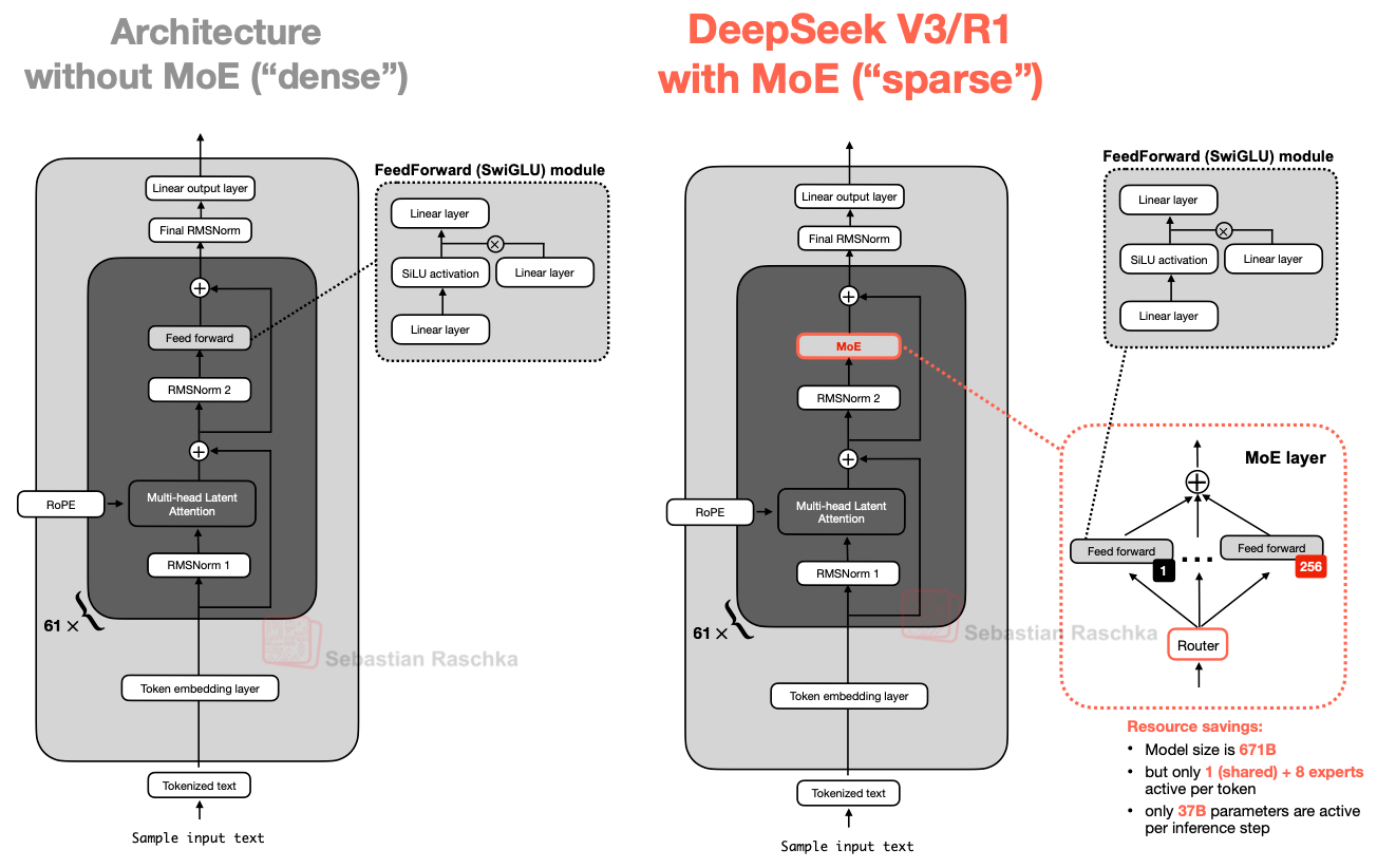
| Total Parameters | 671 billion | Largest open-weight model | Massive knowledge capacity |
| Active Parameters | 37 billion | Only 5.5% activated | Efficiency of 70B model |
| Training Compute | 2.788M H800 hours | 10x less than GPT-4 estimate | $5.5M training cost |
| Training Data | 14.8 trillion tokens | Extreme data efficiency | 22x tokens/parameter ratio |
| Context Length | 128K tokens | Full attention (no sliding) | Novel-length understanding |
Training Innovations
FP8 Mixed Precision Training
DeepSeek V3 pioneered FP8 training at scale, reducing memory and compute requirements by 50% compared to FP16/BF16:
FP8 Format (E4M3) Specification
┌─────────┬──────────────┬─────────────┐
│  Sign   │   Exponent   │   Mantissa  │
│  1 bit  │    4 bits    │    3 bits   │
├─────────┼──────────────┼─────────────┤
│    S    │    E E E E   │   M M M     │
└─────────┴──────────────┴─────────────┘

Range:     2^-6 to 2^8
Precision: ~1.5 decimal digits
Total:     8 bits per value
| Component | Configuration | Purpose |
|---|---|---|
| Gradients | FP8 with gradient scaling | Reduces memory bandwidth by 50% |
| Optimizer States | FP32 (full precision) | Critical for convergence stability |
| Activations | FP8 with per-tensor scaling | Balances range and precision |
| Weights | FP8 with per-channel quantization | Maintains model capacity |
Performance Benchmarks
| Benchmark | DeepSeek-R1 | GPT-4 | Claude 3.5 | Open Model SOTA |
|---|---|---|---|---|
| MMLU (Knowledge) | 87.1% | 86.4% | 88.3% | 79.5% (Llama 3) |
| MATH-500 (Math) | 97.3% | 74.6% | 78.3% | 51.0% (Qwen2) |
| AIME 2024 (Competition Math) | 79.8% | 53.6% | 61.6% | 41.6% (Llama 3) |
| HumanEval (Coding) | 92.7% | 87.2% | 92.0% | 84.1% (Qwen2) |
| GPQA Diamond (Science) | 71.5% | 50.7% | 65.0% | 48.7% (Llama 3) |
Deployment and Serving Optimizations
Production Serving Configuration
Hardware Requirements:
• Minimum: 8x A100 80GB for INT8 inference
• Recommended: 16x H100 80GB for FP16 inference
• Budget option: 32x RTX 4090 with expert offloading
Optimization Techniques:
• KV cache compression via MLA: 8x reduction
• Expert caching: Keep top 32 experts in GPU memory
• Dynamic batching: Group by selected experts
• Speculative decoding: Use smaller model for drafting
Performance Metrics:
• Throughput: 147 tokens/second (batch=32)
• Latency: 12ms per token (batch=1)
• Memory: 320GB for model + 40GB KV cache
Part 4: Model-by-Model Deep Analysis
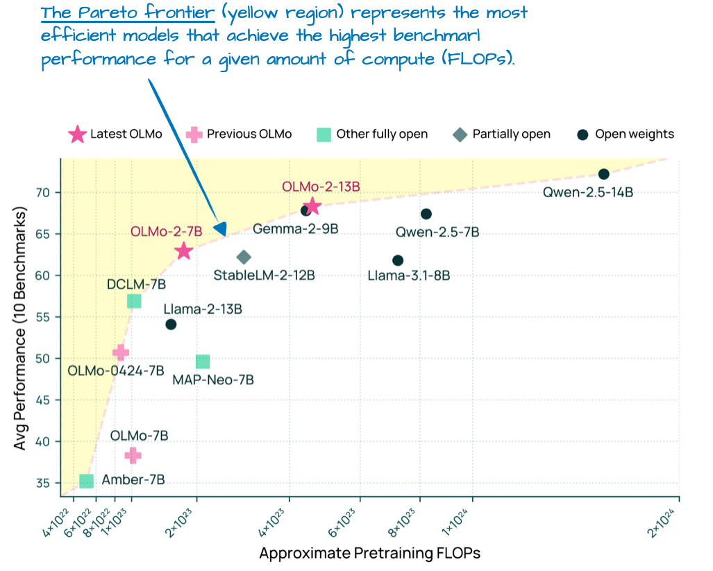
OLMo 2: The Transparent Blueprint
OLMo 2, developed by the Allen Institute for AI, provides unprecedented transparency in LLM development. Every decision, experiment, and failure is documented, making it an invaluable learning resource.
OLMo 2 Technical Specifications
Model Sizes: 1.2B, 7B, 13B parameters
Architecture Details (7B model):
• Hidden dimension: 4,096
• Layers: 32
• Attention heads: 32
• Grouped-Query: 8 KV heads
• Context length: 8,192 tokens
• Activation: SwiGLU
Training Details:
• Tokens: 4 trillion (7B model)
• Batch size: 4M tokens
• Learning rate: 3e-4 peak
• Warmup: 2000 steps
• Hardware: 512x A100 40GB
Normalization Innovation: The Best of Both Worlds
OLMo 2's key contribution is its hybrid normalization approach, combining benefits of Pre-Norm and Post-Norm:
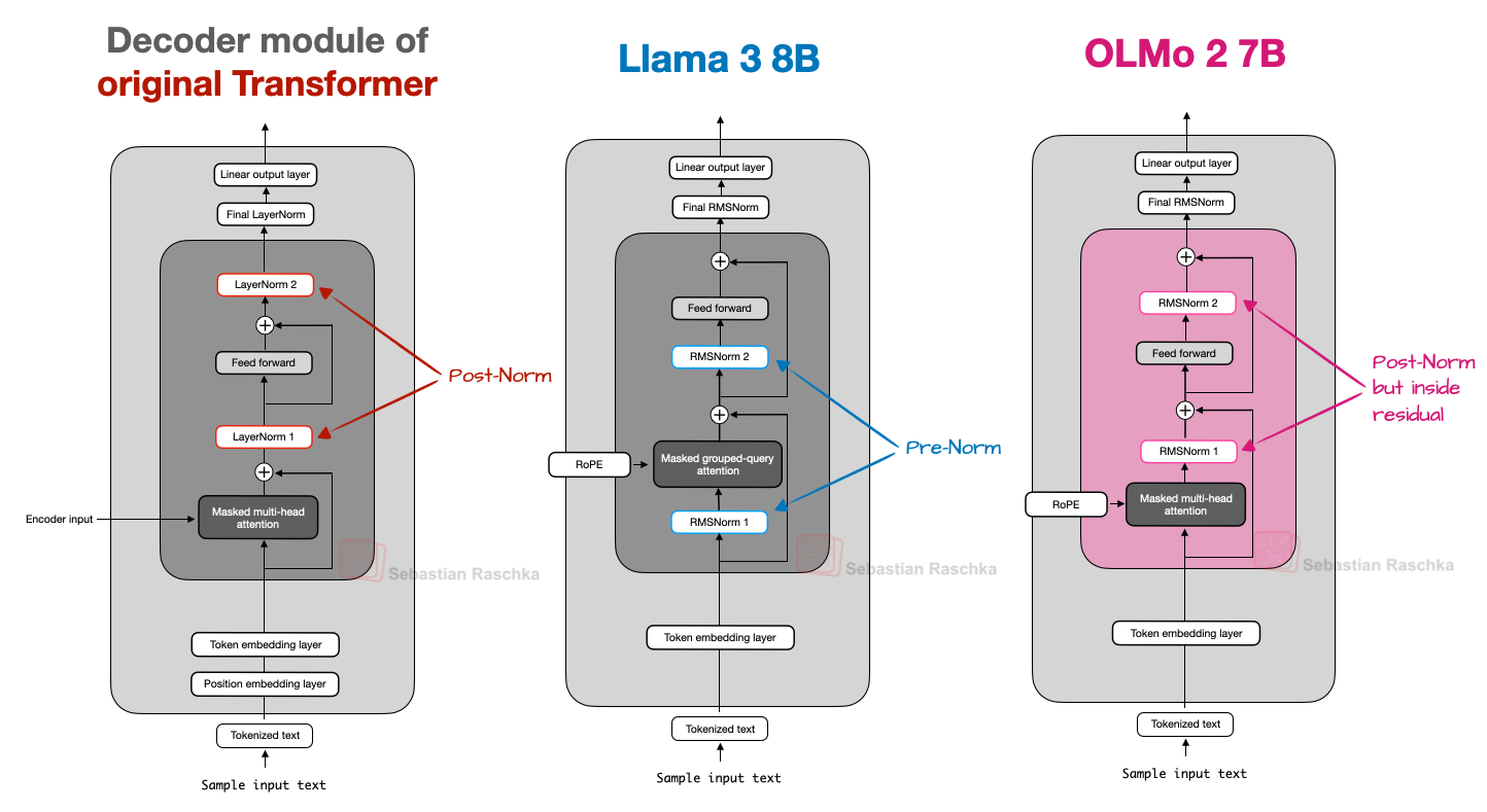
Normalization Mathematics
Standard Pre-Norm (used by most models):
y = x + Attention(LayerNorm(x))
z = y + FFN(LayerNorm(y))
Standard Post-Norm (original transformer):
y = LayerNorm(x + Attention(x))
z = LayerNorm(y + FFN(y))
OLMo 2 Hybrid:
y = LayerNorm(x) + Attention(LayerNorm(x))
z = LayerNorm(y) + FFN(LayerNorm(y))
Key insight: Normalized residual path prevents gradient explosion
while maintaining representational capacity
Gemma 3: Google's Efficiency Champion
Gemma 3 focuses on deployment efficiency rather than pushing parameter counts, optimizing for real-world usage constraints.
Gemma 3 Architecture (27B Model)
Core Specifications:
• Parameters: 27B dense (no MoE)
• Hidden dimension: 3,584
• Layers: 46
• Attention heads: 32 (16 KV heads with GQA)
• Context: 8K training, 1M+ inference via RoPE scaling
Sliding Window Configuration:
• Window size: 4,096 tokens
• Global layers: Every 5th layer (9 total)
• Local layers: 37 layers
• Effective context: Full 8K with 80% less memory
Llama 4: Meta's MoE Evolution
Llama 4 represents Meta's embrace of sparse architectures after the dense-only Llama 1-3 series:
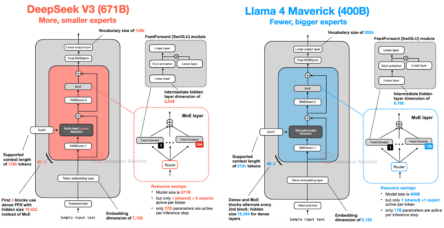
| Aspect | Llama 4 Maverick | DeepSeek V3 | Design Philosophy |
|---|---|---|---|
| Total Parameters | 400B | 671B | DeepSeek: Maximum capacity |
| Active Parameters | 17B | 37B | Llama: Minimize latency |
| Expert Count | 64 | 256 | DeepSeek: Fine specialization |
| Attention Type | GQA (8 groups) | MLA (512d latent) | Llama: Proven reliability |
| Training Data | 15T tokens | 14.8T tokens | Similar scale, different mix |
SmolLM3: Extreme Efficiency at Small Scale
SmolLM3 demonstrates that architectural innovations benefit small models too:
SmolLM3: State-of-the-Art Under 2B Parameters
Model Sizes: 135M, 360M, 1.7B parameters
Key Innovations:
• Deeper than wide: 30 layers for 1.7B model (typical: 24)
• Aggressive GQA: 4 KV heads for 32 Q heads (8:1 ratio)
• Trained on 15T tokens (10,000x parameters!)
• Knowledge distillation from larger models
Performance:
• Matches GPT-3.5 on many tasks at 100x fewer parameters
• Runs on smartphones with 2GB RAM
• 1000+ tokens/second on Apple M2
Qwen3: Specialized Architecture Variants
The Qwen family demonstrates how architectural choices can be tailored for specific use cases:
| Model Variant | Architecture | Optimization | Use Case |
|---|---|---|---|
| Qwen3-72B | Dense + GQA | Quality-first | General purpose |
| Qwen3-VL | Vision encoder + LLM | Multimodal fusion | Image understanding |
| Qwen3-Code | Extended context (32K) | Code-specific tokenizer | Programming |
| Qwen3-Math | Specialized FFN | Symbolic reasoning | Mathematics |
Part 5: Implementation Guide
Building Key Components from Scratch
Let's implement the core architectural innovations to understand them deeply:
1. Grouped-Query Attention Implementation
import torch
import torch.nn as nn
import torch.nn.functional as F
import math

class GroupedQueryAttention(nn.Module):
    """
    Grouped-Query Attention as used in Llama 2/3, reducing KV cache by sharing
    keys and values across groups of query heads.
    """
    def __init__(self, d_model, n_heads, n_kv_heads, dropout=0.1):
        super().__init__()
        assert n_heads % n_kv_heads == 0, "n_heads must be divisible by n_kv_heads"

        self.d_model = d_model
        self.n_heads = n_heads
        self.n_kv_heads = n_kv_heads
        self.n_rep = n_heads // n_kv_heads  # Repetition factor
        self.head_dim = d_model // n_heads

        # Projections
        self.w_q = nn.Linear(d_model, n_heads * self.head_dim, bias=False)
        self.w_k = nn.Linear(d_model, n_kv_heads * self.head_dim, bias=False)
        self.w_v = nn.Linear(d_model, n_kv_heads * self.head_dim, bias=False)
        self.w_o = nn.Linear(n_heads * self.head_dim, d_model, bias=False)

        self.dropout = nn.Dropout(dropout)

    def forward(self, x, mask=None, cache_k=None, cache_v=None):
        batch_size, seq_len, _ = x.shape

        # Compute Q, K, V
        q = self.w_q(x).view(batch_size, seq_len, self.n_heads, self.head_dim)
        k = self.w_k(x).view(batch_size, seq_len, self.n_kv_heads, self.head_dim)
        v = self.w_v(x).view(batch_size, seq_len, self.n_kv_heads, self.head_dim)

        # Transpose for attention: [batch, heads, seq_len, head_dim]
        q = q.transpose(1, 2)
        k = k.transpose(1, 2)
        v = v.transpose(1, 2)

        # Handle KV cache for inference
        if cache_k is not None:
            k = torch.cat([cache_k, k], dim=2)
            v = torch.cat([cache_v, v], dim=2)

        # Repeat K, V to match number of Q heads
        if self.n_rep > 1:
            k = k.repeat_interleave(self.n_rep, dim=1)
            v = v.repeat_interleave(self.n_rep, dim=1)

        # Scaled dot-product attention
        scores = torch.matmul(q, k.transpose(-2, -1)) / math.sqrt(self.head_dim)

        if mask is not None:
            scores = scores.masked_fill(mask == 0, -1e9)

        attn_weights = F.softmax(scores, dim=-1)
        attn_weights = self.dropout(attn_weights)

        # Apply attention to values
        attn_output = torch.matmul(attn_weights, v)

        # Reshape and project output
        attn_output = attn_output.transpose(1, 2).contiguous()
        attn_output = attn_output.view(batch_size, seq_len, -1)
        output = self.w_o(attn_output)

        return output, (k, v) if cache_k is not None else None

# Example usage
model = GroupedQueryAttention(d_model=4096, n_heads=32, n_kv_heads=8)
x = torch.randn(2, 1024, 4096)  # [batch, seq_len, d_model]
output, _ = model(x)
print(f"Output shape: {output.shape}")  # [2, 1024, 4096]
print(f"Memory saved: {(32/8):.1f}x reduction in KV cache")
2. Mixture of Experts Layer
class MoELayer(nn.Module):
    """
    Mixture of Experts layer with top-k routing and load balancing.
    """
    def __init__(self, d_model, d_ff, n_experts, n_experts_per_tok, dropout=0.1):
        super().__init__()
        self.d_model = d_model
        self.n_experts = n_experts
        self.n_experts_per_tok = n_experts_per_tok

        # Router (gate)
        self.router = nn.Linear(d_model, n_experts, bias=False)

        # Experts (simple FFN for this example)
        self.experts = nn.ModuleList([
            nn.Sequential(
                nn.Linear(d_model, d_ff, bias=False),
                nn.SiLU(),  # SwiGLU activation
                nn.Linear(d_ff, d_model, bias=False),
                nn.Dropout(dropout)
            ) for _ in range(n_experts)
        ])

    def forward(self, x):
        batch_size, seq_len, d_model = x.shape
        x_flat = x.view(-1, d_model)  # [batch * seq_len, d_model]

        # Compute router scores
        router_logits = self.router(x_flat)  # [batch * seq_len, n_experts]
        router_probs = F.softmax(router_logits, dim=-1)

        # Select top-k experts per token
        topk_probs, topk_indices = torch.topk(
            router_probs, self.n_experts_per_tok, dim=-1
        )

        # Normalize top-k probabilities
        topk_probs = topk_probs / topk_probs.sum(dim=-1, keepdim=True)

        # Initialize output
        output = torch.zeros_like(x_flat)

        # Route tokens to experts
        for i in range(self.n_experts_per_tok):
            # Get expert index for each token
            expert_idx = topk_indices[:, i]
            expert_weight = topk_probs[:, i].unsqueeze(-1)

            # Process each expert
            for expert_id in range(self.n_experts):
                # Find tokens routed to this expert
                mask = (expert_idx == expert_id)
                if mask.any():
                    token_indices = mask.nonzero(as_tuple=True)[0]
                    expert_input = x_flat[token_indices]
                    expert_output = self.experts[expert_id](expert_input)

                    # Weighted sum
                    output[token_indices] += expert_weight[token_indices] * expert_output

        # Reshape back
        output = output.view(batch_size, seq_len, d_model)

        # Compute load balancing loss (auxiliary)
        # This encourages uniform expert usage
        expert_usage = router_probs.mean(dim=0)  # Average prob per expert
        load_balance_loss = self.n_experts * (expert_usage * expert_usage).sum()

        return output, load_balance_loss

# Example usage
moe = MoELayer(d_model=768, d_ff=3072, n_experts=8, n_experts_per_tok=2)
x = torch.randn(2, 512, 768)
output, aux_loss = moe(x)
print(f"Output shape: {output.shape}")  # [2, 512, 768]
print(f"Load balance loss: {aux_loss:.4f}")
3. Multi-Head Latent Attention (Simplified)
class MultiHeadLatentAttention(nn.Module):
    """
    Multi-Head Latent Attention as used in DeepSeek V3.
    Compresses KV into latent space before caching.
    """
    def __init__(self, d_model, n_heads, d_latent, dropout=0.1):
        super().__init__()
        self.d_model = d_model
        self.n_heads = n_heads
        self.d_latent = d_latent
        self.head_dim = d_model // n_heads

        # Query projection (standard)
        self.w_q = nn.Linear(d_model, n_heads * self.head_dim, bias=False)

        # Latent compression for KV
        self.w_latent = nn.Linear(d_model, d_latent, bias=False)

        # Latent to KV projections (per head)
        self.latent_to_k = nn.Linear(d_latent, n_heads * self.head_dim, bias=False)
        self.latent_to_v = nn.Linear(d_latent, n_heads * self.head_dim, bias=False)

        # Output projection
        self.w_o = nn.Linear(n_heads * self.head_dim, d_model, bias=False)

        self.dropout = nn.Dropout(dropout)

    def forward(self, x, mask=None):
        batch_size, seq_len, _ = x.shape

        # Compute queries
        q = self.w_q(x).view(batch_size, seq_len, self.n_heads, self.head_dim)
        q = q.transpose(1, 2)  # [batch, n_heads, seq_len, head_dim]

        # Compress to latent space
        latent = self.w_latent(x)  # [batch, seq_len, d_latent]

        # Project from latent to K, V
        k = self.latent_to_k(latent).view(batch_size, seq_len, self.n_heads, self.head_dim)
        v = self.latent_to_v(latent).view(batch_size, seq_len, self.n_heads, self.head_dim)
        k = k.transpose(1, 2)
        v = v.transpose(1, 2)

        # Standard attention computation
        scores = torch.matmul(q, k.transpose(-2, -1)) / math.sqrt(self.head_dim)

        if mask is not None:
            scores = scores.masked_fill(mask == 0, -1e9)

        attn_weights = F.softmax(scores, dim=-1)
        attn_weights = self.dropout(attn_weights)

        attn_output = torch.matmul(attn_weights, v)
        attn_output = attn_output.transpose(1, 2).contiguous()
        attn_output = attn_output.view(batch_size, seq_len, -1)

        output = self.w_o(attn_output)

        # For caching, we only need to store the latent representation!
        cache_size = latent.shape[-1]  # d_latent instead of n_heads * head_dim * 2
        compression_ratio = (2 * self.n_heads * self.head_dim) / self.d_latent

        return output, latent  # Return latent for caching

# Example usage
mla = MultiHeadLatentAttention(d_model=4096, n_heads=32, d_latent=512)
x = torch.randn(2, 1024, 4096)
output, latent_cache = mla(x)
print(f"Output shape: {output.shape}")  # [2, 1024, 4096]
print(f"Latent cache shape: {latent_cache.shape}")  # [2, 1024, 512]
print(f"Compression ratio: {(32*128*2)/512:.1f}x")  # ~16x compression
4. RoPE (Rotary Position Embeddings)
class RotaryPositionEmbedding(nn.Module):
    """
    Rotary Position Embedding (RoPE) as used in most modern LLMs.
    """
    def __init__(self, dim, max_seq_len=8192, base=10000):
        super().__init__()
        self.dim = dim
        self.max_seq_len = max_seq_len
        self.base = base

        # Precompute rotation frequencies
        inv_freq = 1.0 / (base ** (torch.arange(0, dim, 2).float() / dim))
        self.register_buffer("inv_freq", inv_freq)

        # Precompute cos and sin for all positions
        self._precompute_cache()

    def _precompute_cache(self):
        seq_idx = torch.arange(self.max_seq_len, dtype=self.inv_freq.dtype)
        freqs = torch.outer(seq_idx, self.inv_freq)

        # Create rotation matrix elements
        emb = torch.cat((freqs, freqs), dim=-1)
        self.register_buffer("cos_cached", emb.cos()[None, None, :, :])
        self.register_buffer("sin_cached", emb.sin()[None, None, :, :])

    def forward(self, q, k):
        # q, k: [batch, n_heads, seq_len, head_dim]
        batch_size, n_heads, seq_len, head_dim = q.shape

        # Apply rotary embeddings
        cos = self.cos_cached[:, :, :seq_len, :]
        sin = self.sin_cached[:, :, :seq_len, :]

        # Rotate half pattern (more efficient than complex number rotation)
        q_rot = self._rotate_half(q)
        k_rot = self._rotate_half(k)

        q_embed = q * cos + q_rot * sin
        k_embed = k * cos + k_rot * sin

        return q_embed, k_embed

    def _rotate_half(self, x):
        """Rotates half the hidden dims of the input."""
        x1, x2 = x.chunk(2, dim=-1)
        return torch.cat((-x2, x1), dim=-1)

# Example usage
rope = RotaryPositionEmbedding(dim=128)
q = torch.randn(2, 32, 1024, 128)  # [batch, heads, seq_len, head_dim]
k = torch.randn(2, 32, 1024, 128)
q_rotated, k_rotated = rope(q, k)
print(f"Q shape after RoPE: {q_rotated.shape}")
Implementation Best Practices
1. Mixed Precision Training: Always enable torch.autocast for automatic mixed precision, providing 2× memory savings and 1.5-2× speedup with minimal code changes.
2. Memory Optimization: Implement gradient checkpointing in memory-constrained environments to trade computation for memory, enabling training of models 2-3× larger.
3. Attention Acceleration: Deploy Flash Attention v2 for 2-3× speedup on long sequences, with automatic handling of causal masking and dropout.
4. Performance Profiling: Use torch.profiler systematically to identify bottlenecks, focusing on data loading, attention computation, and gradient synchronization.
5. Distributed Training: Choose FSDP for simpler setup or DeepSpeed for maximum control over sharding strategies and optimization techniques.
Part 6: Performance Analysis and Benchmarks
Comprehensive Performance Comparison
| Model | Parameters | Active Params | MMLU | HumanEval | MATH | Throughput (tok/s) |
|---|---|---|---|---|---|---|
| GPT-4 | ~1.8T (est) | ~1.8T | 86.4% | 87.2% | 74.6% | ~20 |
| DeepSeek-V3 | 671B | 37B | 87.1% | 92.7% | 97.3% | 147 |
| Llama 4 (70B) | 70B | 70B | 79.5% | 84.1% | 51.0% | 89 |
| Gemma 3 (27B) | 27B | 27B | 75.2% | 76.3% | 42.3% | 215 |
| Qwen3 (72B) | 72B | 72B | 83.0% | 86.1% | 68.2% | 95 |
| OLMo 2 (13B) | 13B | 13B | 67.5% | 65.8% | 28.4% | 312 |
Memory Efficiency Deep Dive
| Component | Standard (MHA) | GQA (4x) | MLA (DeepSeek) | Sliding Window |
|---|---|---|---|---|
| KV Cache/token | 256 KB | 64 KB | 4 KB | 32 KB |
| 32K context memory | 8 GB | 2 GB | 128 MB | 1 GB |
| Max context (40GB) | 160K tokens | 640K tokens | 10M tokens | 1.25M tokens |
| Decode latency | 12ms | 12ms | 15ms | 10ms |
Training Efficiency Analysis
Compute Requirements Comparison
| Model | GPU Hours | Training Cost | Data Size | Infrastructure |
|---|---|---|---|---|
| DeepSeek V3 671B parameters |
2.788M H800 hours | ~$5.5M at $2/hour |
14.8T tokens | 2 months 2,048 GPUs |
| GPT-4 Estimated |
25-50M A100 hours | $50-100M | ~13T tokens | 3-6 months 10,000+ GPUs |
| Llama 3 405B parameters |
30.84M H100 hours | ~$60M | 15T tokens | 4 months 16,000 GPUs |
DeepSeek V3 achieves comparable performance to GPT-4 with 10× less compute, demonstrating the power of architectural efficiency over brute force scaling.
Scaling Laws and Efficiency
Chinchilla Scaling Laws vs. MoE Reality
Chinchilla optimal: N_params = 20 × N_tokens
For 10T tokens: 500B parameters optimal
MoE adjustment: N_active = 20 × N_tokens
For 10T tokens with MoE:
• 500B active parameters needed
• Can achieve with 5T total params at 10% activation
• Or 2T params at 25% activation
DeepSeek V3 validation:
• 14.8T tokens → 296B params optimal
• Has 37B active (underparameterized by 8x)
• Compensates with 671B total capacity
• Result: Beats dense models at same active size
Part 7: Architectural Failures and Lessons Learned
Major Architectural Experiments That Failed
1. Linear Attention (2020-2021)
The Promise: O(n) complexity instead of O(n²) by using kernel approximations.
What Happened: Models like Linformer and Performer showed promise on benchmarks but failed catastrophically on real tasks requiring precise attention (like copying or arithmetic).
The Fatal Flaw: Approximating attention destroyed the model's ability to form sharp, precise connections between tokens.
Lesson Learned: Some computational costs are fundamental—you can't approximate away the need for precise token relationships.
2. Infinite Context via Compression (2023)
The Idea: Compress past context into a fixed-size memory bank updated at each step.
Implementation: Google's Infini-Transformer, Anthropic's experiments with compression.
What Failed: Information bottleneck—compressing 100K tokens into 1K dimensional vector loses critical details.
Current Status: Abandoned in favor of sliding windows and efficient KV caching.
3. Adaptive Computation Time (2021-2022)
The Concept: Let the model decide how many layers to use per token—simple tokens use fewer layers.
The Problem: Training instability—gradients became chaotic when different tokens used different depths.
Why It Failed: Batching nightmare—can't efficiently batch tokens using different computation paths.
Legacy: Inspired MoE's token-routing, but with fixed depth.
4. Extreme Sparsity: 512+ Experts (2023)
ByteDance's Experiment: If 256 experts work well, why not 512 or 1024?
What Broke:
• Router collapse—couldn't distinguish between hundreds of similar experts
• Memory explosion—model wouldn't fit on any realistic cluster
• Load balancing impossible—some experts never activated
The Discovery: Natural language has ~200-300 distinct "skill clusters"—more experts don't help.
5. Hierarchical Transformers (2020-2021)
The Vision: Process text at multiple granularities—characters, words, sentences, paragraphs.
Implementations: Funnel Transformer, Hourglass Transformer.
The Failure: Information loss at compression points destroyed fine-grained understanding.
Why It Matters: Led to the insight that flat architectures with uniform resolution are optimal.
Lessons from Failed Optimization Attempts
| Optimization | Promise | Reality | Lesson |
|---|---|---|---|
| 8-bit Quantization (Weights) | 4x memory reduction | 2-5% accuracy loss | Acceptable for inference, not training |
| 4-bit Quantization | 8x memory reduction | 10-20% accuracy loss | Only viable with QLoRA fine-tuning |
| Pruning (90% sparsity) | 10x speedup | Destroys emergent abilities | LLMs need redundancy for robustness |
| Knowledge Distillation | 10x smaller model | Loses reasoning ability | Compression destroys chain-of-thought |
| Mixture of Depths | Adaptive computation | Training instability | Fixed depth with sparse width better |
Critical Insights from Failures
1. Attention is Irreducible: Every attempt to approximate attention (linear, compressed, hierarchical) has failed. The O(n²) complexity appears fundamental.
2. Sparsity Has Limits: MoE works because it's sparse in width (experts) not depth (layers). Sparse depth breaks gradient flow.
3. Quantization Ceiling: Below 8 bits, models lose emergent abilities. There's a fundamental precision requirement for intelligence.
4. Scale Enables Efficiency: Counterintuitively, larger sparse models are more efficient than smaller dense ones at the same performance level.
Part 8: Global Innovation Patterns
The Geography of LLM Innovation
The development of large language models has become a global endeavor, with different regions contributing unique innovations shaped by their constraints and priorities:
Regional Innovation Patterns
| Region | Focus Areas | Approach | Key Innovations |
|---|---|---|---|
| United States OpenAI, Anthropic, Meta |
Capability frontiers, safety research | Massive compute budgets, closed models "Scale first, optimize later" |
RLHF, constitutional AI, chain-of-thought |
| China DeepSeek, Alibaba, Baidu |
Efficiency, open-source leadership | Algorithmic innovation under hardware constraints "Do more with less" |
MLA, extreme MoE, FP8 training |
| Europe Mistral, Aleph Alpha |
Specialized models, privacy-preserving AI | Efficient architectures for specific domains "Quality over quantity" |
Mixture of experts at small scale |
| Middle East Falcon, Jais |
Multilingual models, regional languages | Large-scale training with oil-funded compute "Sovereignty through AI" |
Multiquery attention, RefinedWeb dataset |
How Hardware Constraints Drive Innovation
The GPU Export Restrictions Paradox
US restrictions on high-end GPU exports to China (A100, H100 banned) inadvertently accelerated Chinese AI innovation. These hardware constraints forced engineers to develop breakthrough efficiency techniques that now benefit the entire AI community.
How Constraints Drove Innovation: Limited memory availability led to the invention of Multi-Head Latent Attention (MLA) achieving 8× compression. Fewer available GPUs catalyzed the pioneering of FP8 training methods with 2× speedup. High serving costs motivated the creation of extreme Mixture of Experts architectures delivering 10× efficiency improvements. The fundamental principle emerged: when you can't buy more hardware, you must optimize algorithms.
Result: DeepSeek V3 matches GPT-4 with 10× less compute, proving that necessity truly drives innovation.
Open Source vs. Closed Source Dynamics
| Aspect | Closed (OpenAI, Anthropic) | Open (DeepSeek, Meta) | Impact |
|---|---|---|---|
| Innovation Speed | Slower, careful | Rapid iteration | Open models catch up in 6-12 months |
| Safety Research | Extensive, private | Community-driven | Different approaches to alignment |
| Reproducibility | Zero | Full | Enables scientific progress |
| Cost to Users | $15-60/M tokens | $0 (self-host) | Democratizes access |
| Customization | Limited to API | Full control | Enables domain-specific models |
Part 9: Future Directions
Emerging Architectural Trends
1. Hybrid Attention Mechanisms
Future models will likely combine multiple attention patterns dynamically, adapting to the specific requirements of each input. Local attention will handle syntax and grammar processing where nearby token relationships dominate. Global attention mechanisms will engage for long-range reasoning tasks requiring full context awareness. Compressed attention variants will optimize memory efficiency for resource-constrained deployments, while cross-attention layers will enable seamless multimodal fusion between text, images, and other modalities.
Research Direction: The key innovation will be learning to route between attention types based on content characteristics, similar to how MoE architectures route tokens to specialized FFN experts. This content-aware routing could reduce computational costs by 70% while maintaining full model capabilities.
2. Extreme Sparsity: The 1% Activation Goal
Current MoE models activate 4-9% of parameters per token, but the next frontier pushes toward 1% activation rates. This will be achieved through hierarchical routing that first selects expert clusters before individual experts, dynamic expert creation that grows specialized modules as needed during training, and conditional computation that intelligently skips entire layers when their contribution would be minimal.
Challenge: Maintaining gradient flow and training stability with extreme sparsity remains the primary technical obstacle, requiring novel optimization techniques and careful architectural design.
3. Beyond Transformers: Hybrid Architectures
While transformers dominate current architectures, hybrid models are emerging that combine the best of multiple paradigms. Mamba + Transformer hybrids achieve linear complexity for routine token processing while reserving quadratic attention for critical reasoning steps. RetNet + Transformer architectures leverage retention mechanisms for efficient memory management alongside attention for complex reasoning. RWKV + Transformer models blend RNN-like efficiency with transformer-quality outputs, achieving the best of both worlds.
Key Insight: Different architectural components excel at different cognitive tasks—future models will intelligently combine these components, dynamically selecting the right tool for each subtask within a single forward pass.
The Path to 100 Trillion Parameters
Scaling Projections
Assuming current trends continue:
2024: ~1T parameters (DeepSeek V3 at 671B)
2025: ~5T parameters (rumored GPT-5 scale)
2026: ~20T parameters
2027: ~100T parameters
Required innovations for 100T scale:
• <1% parameter activation (currently 5%)
• Hierarchical MoE with 10,000+ experts
• Model parallelism across 100,000+ GPUs
• New hardware: Optical interconnects, 3D chip stacking
• Training: Curriculum learning, progressive growing
Fundamental Questions Remaining
1. Is attention optimal? After 7 years, no better mechanism has been found. Is this fundamental or have we not looked hard enough?
2. What's the limit of sparsity? Can we build models that use 0.1% of parameters per token while maintaining quality?
3. Can we unify architectures? Is there a single architecture that's optimal for all tasks, or will we need specialized architectures?
4. What emerges at 100T scale? Will we see qualitatively new capabilities, or just incremental improvements?
5. How do we achieve sample efficiency? Humans learn language from ~100M words. LLMs need 10,000x more. Why?
Conclusion: The Architecture Convergence
As we survey the landscape of LLM architectures in 2024-2025, a remarkable pattern emerges: despite starting from different philosophies and constraints, the field is converging on a common set of architectural patterns:
The Emergent Consensus
Universal Components (adopted by all):
• Transformer backbone with pre-normalization
• SwiGLU activation functions
• Rotary position embeddings (RoPE)
• Some form of attention optimization (GQA, MLA, or sliding window)
• Mixed precision training (FP8 or BF16)
Divergent Choices (philosophical differences):
• Dense vs. MoE (quality vs. efficiency)
• Number of experts (US: fewer, larger; China: many, smaller)
• Open vs. closed source
• Safety mechanisms vs. capability focus
The evolution from GPT-2 to DeepSeek V3 represents not a revolution but a careful refinement—thousands of small improvements that compound into dramatic gains. The transformer architecture, now seven years old, has proven remarkably robust and scalable.
Perhaps most importantly, the global nature of LLM development—with crucial innovations coming from China, the US, Europe, and beyond—demonstrates that advancing AI is truly a human endeavor. Different constraints breed different innovations, and the diversity of approaches strengthens the field.
As we look toward the future, the path seems clear: continued scaling, increased sparsity, and careful engineering optimization. The age of architectural exploration may be ending, replaced by an age of architectural refinement. The fundamental building blocks are in place; now we build higher.